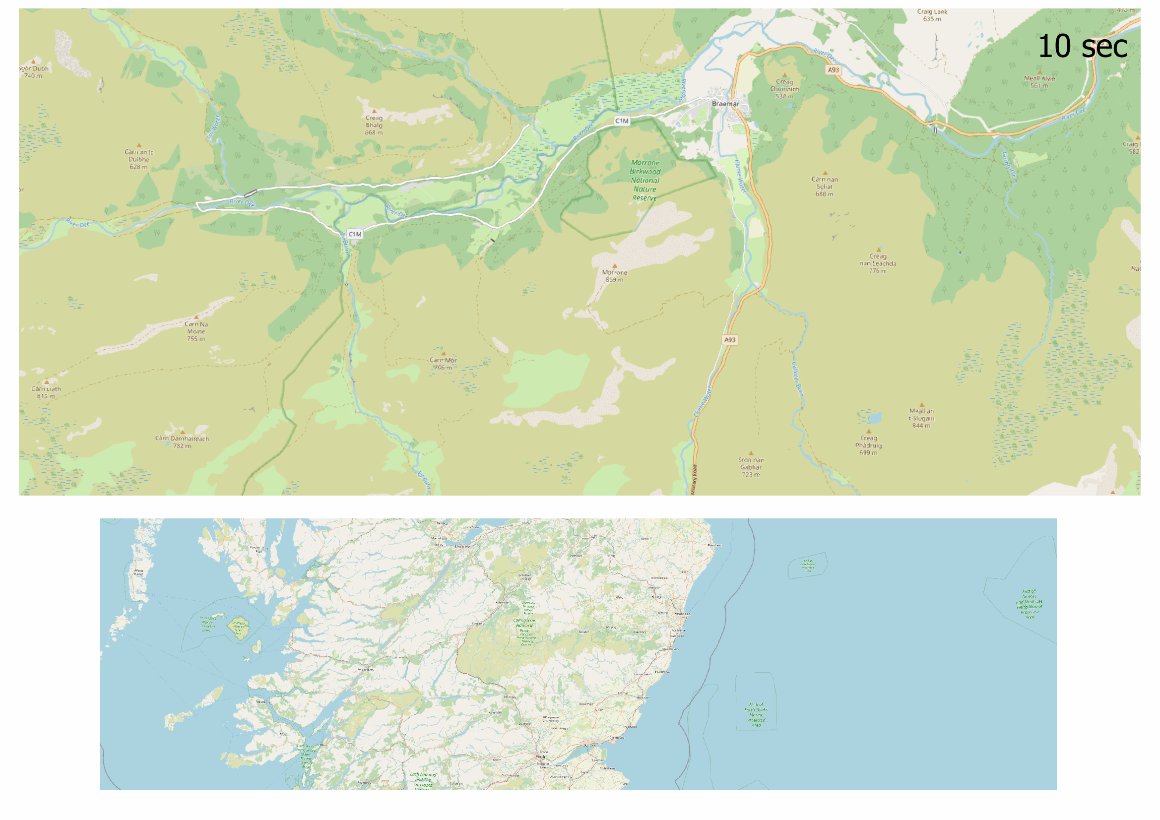
I have been playing around with the excellent Isochrones Service (driving-car) on my local docker install, using a modified Scotland .pbf in which I used osmconvert and osmfilter to exclude highways=tracks because many of these are not accessible to cars.
I’ve noticed some quirks in the isochrone polygons as the range time increases. My approach has been to increment the range time by 10 secs to compare the results, as in this little animated example here:
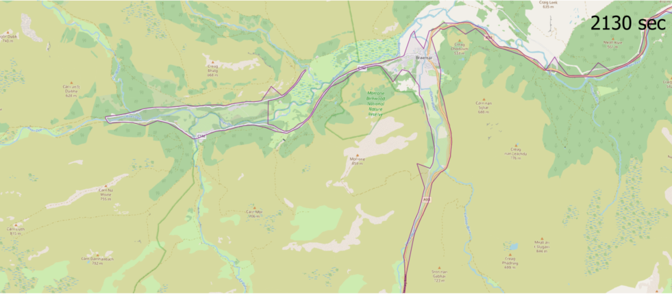
Here’s a good example of the issue: at 2130 seconds the isochrone polygon looks like this
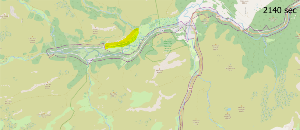
But at 2140 seconds, the next frame looks like this - I’ve highlighted in yellow a section of road that was in the previous frames, but is deleted from future frames even though the starting point is unchanged
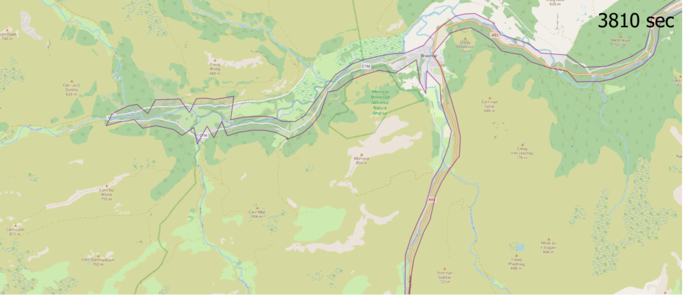
As the range gets even bigger, we see strange artefacts like this, where the isochrone polygon intersects the road network in a slightly unexpected and undesirable way, like at 3810 sec:
Is there an API parameter or ‘ors-config.json’ setting that will prevent the polygons from going weird in he examples above? I appreciate that as my range increases, the number of nodes will increase too, and that some simplification occur. But ideally I’d like to preserve the original road network in the output polygons, so if there’s anything I can do to maintain accuracy please let me know. Thanks
In that case, there is probably no other fix than editing the algorithm code itself.
But it might also be the switch to a different isochrone algorithm for greater ranges.
Could you provide the docker image/ or git commit hash and the configuration of the ors instance you are running and probably the code/commands to reproduce the used osm file from the scotland.pbf?
Generally, the larger an Isochrone gets, the more complex it becomes. The complexity not only affects its spatial form, but also the construction and smoothing of the isochrone in openrouteservice. To avoid having a processing bottleneck with larger Isochrones, they tend to consist of relatively fewer points (relatively speaking, per individual area unit). It’s a balance between accuracy and speed.
Especially in the last image, you can see the effect on the left part, where the upper and lower line look more and more jagged. This is due to less stabilizing points being available.
Make sure to check out the smoothing_factor parameter and its explanation at Dashboard | ORS
and to play around with it a little.